Multi-Agent Reinforcement Learning on Trains

Problem Description

One of the major bottlenecks faced by the transportation and logistic companies around the world right now is the punctuality of all their train operations. Punctuality not only involves regularity in time but also relies on several factors like ensuring safety and providing reliability of service [1]. This project’s main focus is to solve the problem of railway traffic control. Through this project, we aim to work on this domain by shifting solutions from traditional Operations Research techniques to a Reinforcement Learning approach!

We make use of the environment provided in the flatland challenge that is built to tackle this exact problem of scheduling and rescheduling trains. They provide a grid-world environment that will be described in detail over the next section. The major moving parts in this problem, for now, are the trains (which are generally referred to as agents throughout this blog), stations (to which specific trains have to arrive at), and tracks (that form a network that connects different stations).

The goal of this project is not only to make the trains reach their destination without suffering from deadlocks or traffic accidents, but it is also to minimize the time required to reach the destination. Since most of the approaches to solve this problem efficiently were previously based on Operations Research techniques, through this project, we test various single-agent and multi-agent reinforcement learning algorithms and compare their efficiency.

Environment

The environment used for this project can be found here [6]. The major features of this environment are:

Observation Space

There are three forms of observation spaces currently supported by the flatland environment.

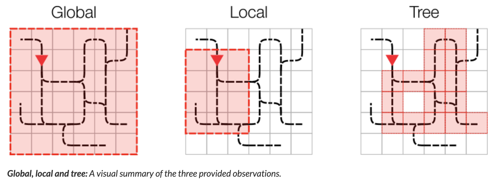
The first observation type is the Global Observation space, which is very similar to the raw-pixel type of observation spaces used in the Atari games, with a slight difference. The global observation space is h x w x c, dimensional where h is the height of the environment, w is the width and c represents the channels. Instead of raw pixel values, each channel (total 5) provides some information about the current state. For example, channel 0 contains the one-hot encoding representation of an agent’s current position and direction, channel 1 contains information about other agent’s position and direction, etc.

The second type is a Local Observation space which is a constrained version of the global observation space.

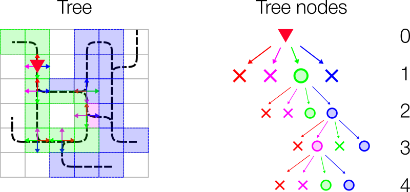
The third observation type is the Tree Observation space, which makes use of the network/graph-like structure of the environment. The tree is 4-ary tree with each node’s 4 child edges representing nodes in the Left, Forward, Right, Backward direction. Each node in the tree consists of 12 features. For training our policy networks, we would need to convert these tree representations into linear forms. This is achieved by a normalization procedure exposed by Flatland. The observation depth of the tree determines the state size as it is equal to the number of leaf nodes of the tree. For example, with an observation depth of 2, we work with a state size of 231.

Action Space

The action space for this problem is discrete having 5 possible options:

0: Do Nothing
1: Deviate Left
2: Go Forward
3: Deviate Right
4: Stop

One thing to note in this environment is that not all actions are possible at any given moment because the agent is restricted by the structure of the network.

Complexity control

This environment contains various properties that can be configured to control the complexity of the resulting network. For this project, the complexity used was simple as we wanted to test the performance of different algorithms in a limited time and resources. Here are the parameters we used for reference:

Property	Description	Complexity value used
malfunction_rate	Poisson rate at which malfunctions happen for an agent	2%
max_num_cities	Maximum number of stations in on observation	2
grid_mode	random vs uniform distribution of cities in a grid	False
max_rails_between_cities	Maximum number of rails connecting cities	2
max_rails_in_city	Maximum number of parallel tracks inside the city	3
observation_tree_depth	The depth of the observation tree	2

Multi-Agent RL

Reinforcement learning has been successfully applied to solving tasks in various fields such as game playing and robotics [7]. However, the most successful settings have predominantly been single-agent systems, where the behavior of other actors is not taken into account. Like our problem statement, many real-world environments are multi-agent settings that involve interaction between multiple agents. Multi-Agent RL is an active field of research [7] with potentially significant impact on RL in real-world. In this section, we discuss aspects of multi-agent environments that theoretically differentiate between single-agent and multi-agent settings.

Concepts

Markov Games are a multi-agent extension of Markov Decision Processes (MDPs) that are used to model single-agent systems [8]. A Markov Game is tuple \(\langle S, A_1, ..., A_N, O_1, ..., O_N \rangle\) where:

\(N\) = number of agents
\(S\) = set of states (all possible configurations of all agents)
\(A_1, ..., A_N\) = set of actions of the agents
\(O_1, ..., O_N\) = set of observations of the agents

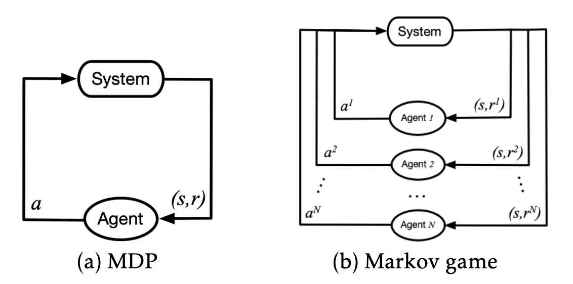
Each agent follows a stochastic policy \(\pi_{\theta_i} : O_i \times A_i \rightarrow [0, 1]\) while transitioning according to the state transition function \(T : S \times A_1 \times ... A_n \rightarrow S\) and receives a reward defined by the reward function \(r_i : S \times A_i \rightarrow \R\). The aim of all agents is to maximize their total expected return \(R_i = \sum_{t = 0}^{T} \gamma^{t} r_i^t\) over time \(T\), with a discount factor \(\gamma \in [0, 1]\).

In contrast to single-agent RL, the value function for every agent is a function of the joint policy. Therefore, intuitively, we can see that the solution of a Markov Game would be different from that of a Markov Decision Process because the optimal policy of an agent may be dependent on the policies of all other agents. One such solution that characterizes the optimal joint policy is the Nash Equilibrium. The equilibrium has been proved to always exist in discounted Markov Games, but may not be unique. MARL algorithms are designed to converge to such an equilibrium.

MARL settings can be mainly characterized into the following:

• Cooperative : agents share a common reward
• Competitive : one agent’s loss is other’s gain; modeled as a zero-sum Markov Game
• Mixed

Challenges

Simultaneous learning by all agents can make the environment non-stationary from the view of a single agent [7]. This is so, since the action taken by one agent can influence the decisions made by others and the evolution of the state. Hence, it is necessary to take into account joint behavior of the agents. This is in contrast with the single-agent setting which violates the stationarity assumption (Markov property).

To account for non-stationarity, we may attempt to tackle MARL from a combinatorial perspective by modeling the joint action space of all agents. Such a modeling exponentially increases the dimension of the action space and is hence cursed by dimensionality. This casuses an issue of scalibilty on the computation side and also complicates theoretical convergence guarantees [7].

Solutions

We explore two paradigms that MARL algorithms employ for overcoming these challenges. The first and a naive approach is to consider all agents independent and learn Q-values for each of them. This approach is known as Independent Q-Learning (IQL). From the view of one single agent, other agents are considered as part of the environment. As we can see intuitively, the algorithm is not learning any explicit co-operation amongst the agents and is not expected to converge. However, in practice, it ends up working quite well in some cases. This suggests the possible use of IQL as baselines for multi-agent systems.

A second and a recently popular approach is based on the principle of Centralized Training and Decentralized Execution. The key trick here is that communication between agents is not restricted during learning, however the individual policies for all agents are limited in communication during execution. Neural networks that learn policies in MARL based on decentralized execution have some explicit components that learn the co-ordination amongst agents. This is a reasonable paradigm because it can also be applied to some real-world settings.

Models

We implemented the above mentioned approaches on our problem. Specifically, we focused on two IQL approaches and two MARL approaches based on decentralized execution. In this section, we briefly describe the algorithms. The reader is encouraged to read the corresponding papers for a greater depth.

Dueling Double Deep Q-Network

Deep Q Networks generally suffer from the bias problem, which refers to the network overestimating the rewards in noisy environments, and it also suffers from the moving target issue, which refers to the usage of the same network for training and evaluation. [2]

To solve this problem Double Deep Q Networks were introduced (DDQN). This algorithm adds another Q network which is known as the target-Q network, and both of these networks are trained by random sampling of data from a fix-sized bank of points known as the replay memory. The introduction of this target network into the algorithm helps curb the moving target problem since both the training and evaluation happens in different networks. It also solves the bias problem due to the usage of replay memory.

The Dueling Deep Q network algorithm uses a different formulation of the Q function. Here, the Q function for a state-action pair is divided into a sum of two terms, the first one being the value function for the state, and the second one being the advantage function for the state-action pair.

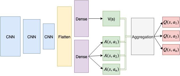
As you can see from the image above, an embedding representation is calculated from the current state which is then fed into one set of dense layers to calculate the value for the state, and another set of dense layers to calculate the advantage of every action on the state under the policy. Instead of simply summing over them, which leads to the problem of identifiability, they are aggregated by subtracting the normalized advantage to the sum of value and advantage per action. This entire pipeline returns the Q values for a state for each possible action.

When the above architecture for Q-value estimator is used along with a similarly constructed target Q-value estimator, and a replay memory, it becomes the Dueling Double Deep-Q Network (D3QN).

Rainbow Deep Q-Network

Rainbow DQN combines the many independent improvements that have been made on the traditional DQN algorithm over the years. This algorithm uses a mixture of Double Q-learning, Prioritized replay, Dueling networks, Multi-step learning, Distributional RL, and Noisy Nets. Double and Dueling networks were described in the previous section. Prioritized replay memory helps sample experiences such that there is more to learn from them. Multistep learning enables using accumulating rewards for n-step (rollout) before storing them, rather than using the single next-step reward. Distributional RL helps to learn the distribution of returns rather than expected returns. Noisy Nets allow the addition of noise to the parameters of the linear layers of the network, which enables “state-conditional exploration with a form of self-annealing” [3]

Multi-Agent Attention Critic

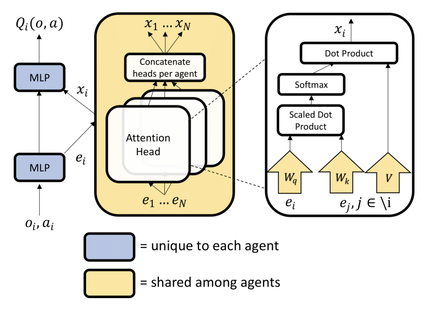
Intuitively, the attention mechanism allows each agent to query other agents for their actions and observations. Therefore, the q-value of an agent is a function of the agents observation and action, as well as of the weighted sum of values of other agents. This function is approximated by a MLP. Attention weights transform the state-action embeddings into keys and queries. A common embedding space of selectors, extractor and keys is made possible by parameter sharing [10].

Multi-Agent Advantage Actor Critic

MAA2C is a simple extension of the single-agent version of Actor Critic model, the only difference being that there is a centralized critic trained while the executing actors are trained per agent. In an actor-critic system, the critic estimates the value function from state-action input while the actor learns a policy via the policy gradient theorem. The advantage function is employed to reduce the variance of the policy gradient and provides better convergence [11].

Experimentation Details

In this section we describe the specific hyperparameters for training our models for reproducibility of results. Note that these experiments were conducted on a small environment. The complexity of the environment is determined by the parameters as described in the Environment section. The experiments were carried on Google Colab using GPU accelerators.

Following are some of the common training parameters used across models:

Parameter	Description	Complexity value used
\(\gamma\)	Discount value	0.99
\(\tau\)	Soft update rate	0.001
batch_size	Batch Size	128
replay_size	Size of Replay Memory	\(10^5\)
n_episodes	Number of episodes	2500
n_agents	Number of agents	2
LR (DDDQN)	Learning Rate for DDDQN	\(5 \times 10^{-4}\)
LR (Rainbow)	Learning Rate for Rainbow DQN	\(5 \times 10^{-4}\)
LR Critic (MAAC)	Learning Rate for the Centralized Critic in MAAC	\(10^{-4}\)
LR Agent (MAAC)	Learning Rate for Agents in MAAC	\(10^{-4}\)
LR Critic (MAA2C)	Learning Rate for the Critic in MAA2C	\(3 \times 10^{-4}\)
LR Agent (MAA2C)	Learning Rate for Agents in MAA2C	\(3 \times 10^{-4}\)
Attention heads	Number of attention heads in MAAC	\(4\)
malfunction_rate	Poisson rate at which malfunctions happen for an agent	2%
max_num_cities	Maximum number of stations in on observation	2
grid_mode	random vs uniform distribution of cities in a grid	False
max_rails_between_cities	Maximum number of rails connecting cities	2
max_rails_in_city	Maximum number of parallel tracks inside the city	3
observation_tree_depth	The depth of the observation tree	2

Results

We present the results from D3QN, Rainbow DQN and MAAC. We report the metric ‘normalized score’ as is used in the Flatland challenge.

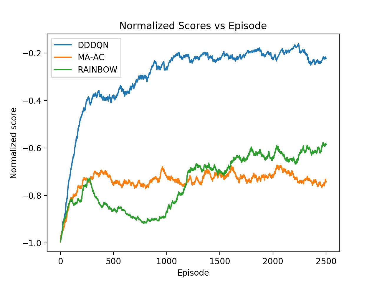
We observe that we get the best performance from the IQL-based DDDQN model. This might be because of the simplicity of the environment, but in general this approach may not scale well with increasing number of agents and increasing complexity of the train network. Note that the Rainbow DQN has not yet reached convergence and do so with more number of episodes. Also, the MAAC policies do not give good results compared to the DQNs. This might might attributable to the number of episodes required for convergence. The original MAAC paper trains agents for over 50k episodes. Since we were limited by resources provided by Google Colab, we could not train our policies for a very long time. From the visualization below, we can also see that the MAAC policy hasn’t converged completely as even the best performing test case isn’t optimal.

DDDQN

Rainbow DQN

MAAC

Future Work

Even though we see that D3QN performs the best on this comparatively simpler multi-agent environment, as discussed in the Results section, this could be because of the lesser complexity of the network. We believe that this can be proved by training on a more complex network for this environment. Some initial experiments do show that D3QNs can’t handle deadlocks as seen in the video above. So, we plan to continue working to improve the results in the following sequence:

1. Make MA-A2C work decently on the simpler network by checking for code bugs and tuning hyperparameters
2. Train MAAC for a larger number of episodes in the order of 10000
3. Test D3QN’s performance on a more complicated network in this environment and compare it with that of MA-A2C and MAAC.

The development for this project can be found here

References

1. Francesco C. et al (2010) “Railway Dynamic Traffic Management in Complex and Densely Used Networks”
2. https://medium.com/analytics-vidhya/introduction-to-dueling-double-deep-q-network-d3qn-8353a42f9e55
3. Matteo H. et al (2017) “Rainbow: Combining Improvements in Deep Reinforcement Learning”
4. https://github.com/Curt-Park/rainbow-is-all-you-need
5. https://github.com/ChenglongChen/pytorch-DRL
6. Flatland Challenge: https://www.aicrowd.com/challenges/flatland-challenge
7. Foerster Jakob N. (2018) “Deep Multi-Agent Reinforcement Learning”
8. Zhang K. et al (2019) “Multi-Agent Reinforcement Learning: A Selective Overview of Theories and Algorithms”
9. Silver D. et al (2015) “Deep Reinforcement Learning with Double Q-learning”
10. Iqbal S. et al (2019) “Actor-Attention-Critic for Multi-Agent Reinforcement Learning”
11. Paczolay G. et al (2020) “A New Advantage Actor-Critic Algorithm For Multi-Agent Environments”